Value Sketches Using k-Means Clustering
All Processing code for this article, along with images, can be found on Github
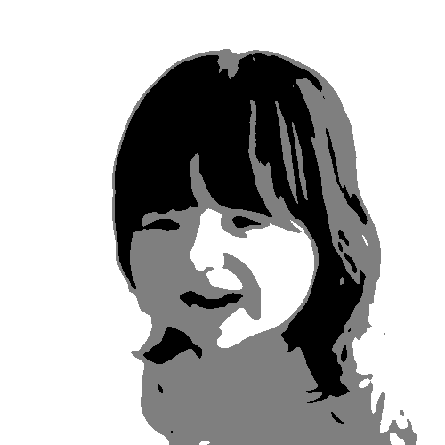
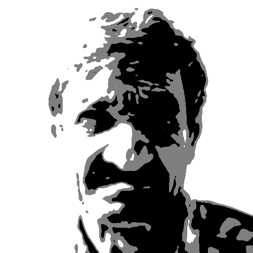
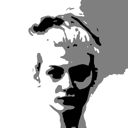
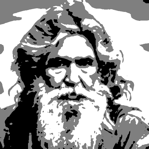
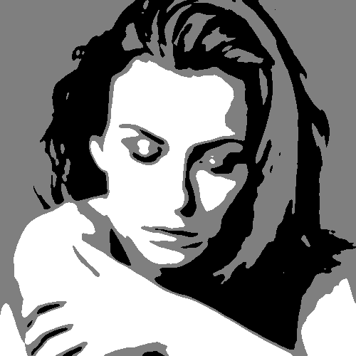
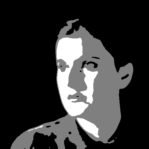
In this post, I explain an algorithm for creating value sketches from images, which are quick sketches based on a few greyscale values used by artists to quickly experiment with compositions. Typically it’s done using three values to give it some depth: a light, dark, and medium tone, and I’m always amazed at how just three values can make a flat shape suddenly appear three dimensional.
I’ll explain in detail how to generate three-value sketches using k-means clustering. For those interested in learning more about this, this technique is called “image segmentation”; the partitioning of an image into multiple segments, or sets of pixels, and k-means clustering is only one of many techniques that can be used to achieve this.
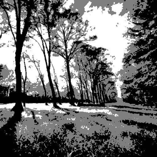
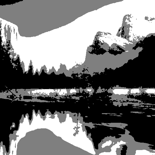
Before we get to the details though, here are some images courtesy of this simple algorithm.
TIP: The reference images used for generating the images below have been taken from Pixabay and Pexels, which are great sources for images licensed under the CC0 license.


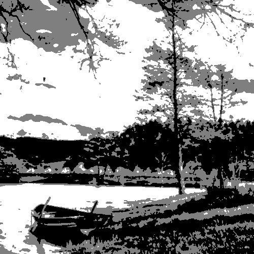
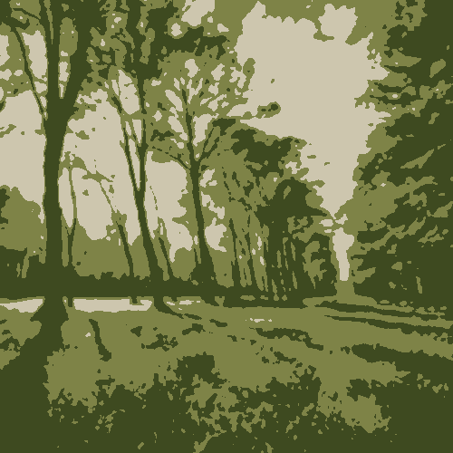
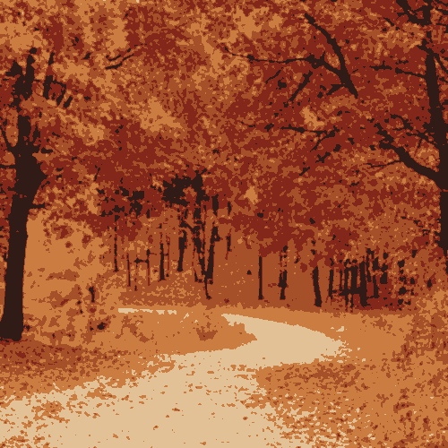
The approach also works fairly well on landscapes, although the level of detail in such images makes it a little more chaotic. Here are a couple of examples below.
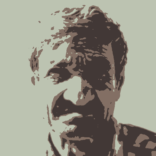
It also works great with colors! Since the approach involves averaging the colors of pixels, the final colors are much more subdued creating a nice, mellow effect.

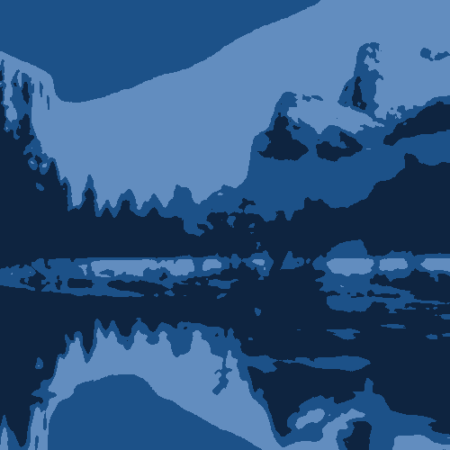
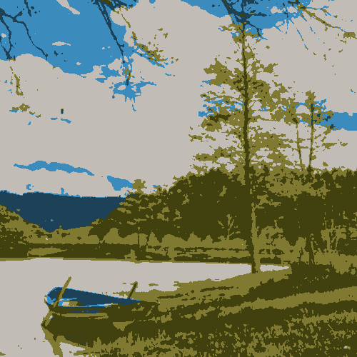
This approach is also of course not limited to just three clusters. Adding more clusters gives more depth and more detail. Here are some examples with five clusters. See if you can identify all the five colors being used!

Overview of the Approach
What the k-means clustering algorithm does is classify some input items into a specified number of clusters using some criteria we specify.
In our case, the input we provide is individual pixels comprising an image. We pick three clusters, one for each of the three tones we want. And the criteria we use for assigning pixels to clusters is the “color distance”; the pixel is assigned to the cluster whose color is closest to its own. This is performed in iterations until no pixel-cluster assignments change.
Note that in our case, the color of the cluster is simply the average color of all pixels assigned to it. (In the beginning since there are no pixels assigned to any cluster, we just pick white as the default.)
At a high level, this is what we’re doing:
function iteration() {
    for every pixel in the image:
        calculate color distance to each cluster
        assign pixel to cluster with lowest found distance
        if cluster assignment changed from last time, make note

    for every cluster:
        re-calculate average color based on new pixel assignments

    return (number of pixels whose assignments changed)
}

// Call iteration() until assignment changes are zero
while (iteration() != 0);
At the end of the k-means iterations, what we end up with are three sets of pixels assigned to three clusters based on their color distance. We map these to black, white, and an intermediate gray value to get our three-value sketches.
Let’s dive into the most complicated bit of this approach, which is the k-means implementation. I show how to do this in Processing but it can of course be applied in any language. The key is to understand the underlying concept.
k-Means Clustering in Processing
Let’s start with a simple KMeansSegmentation class.
class KMeansSegmentation {
  PGraphics image;
  int num_clusters;
  color[] cluster_colors;
  int[][] cluster_assignments;
};
The class contains four variables. The image variable is going to be a
PGraphics instance with our target image and the num_clusters variable
holds the number of clusters we want. The cluster_colors variable is an
array that holds the average color of all pixels assigned to each cluster
(containing num_cluster values). Finally, the cluster_assignments variable
is a two-dimensional array of size widthxheight, one for each pixel, holding
the cluster number assigned to each pixel of the image.
Initially, we provide the class constructor with an image and the number of clusters to create. Since no cluster assignments have been made for any pixels just yet, we assign white as the color of each cluster, and assign an invalid cluster index for each pixel.
class KMeansSegmentation {
  ...
  KMeansSegmentation(PGraphics pg, int n) {
    image = pg;
    num_clusters = n;

    /* Create an array of colors, one for each cluster */
    cluster_colors = new color[num_clusters];

    /* Create a 2D array, one for each pixel of the image */
    cluster_assignments = new int[image.width][image.height];

    /* Assign white as the initial color to all clusters */
    for (int i = 0; i < n; i++)
      cluster_colors[i] = color(255, 255, 255);

    /* Initially assign an invalid cluster index to each pixel */
    for (int x = 0; x <image.width; x++)
      for (int y = 0; y < image.height; y++)
        cluster_assignments[x][y] = -1;
  }
  ...
};
Let’s now get to the main iteration function that we sketched out earlier.
Main Iteration Function
Below is the iteration() function that performs three steps. It first
assigns individual pixels to clusters based on the color distance between them.
Second, it re-calculates the average color of each cluster based on the new
assignments. Finally, it returns the number of pixels whose cluster assignments
changed in this iteration. We invoke the iteration() function until this
reaches zero.
Rather than explain with inline text, I’ve embedded comments for the major parts of the function below. It might look intimidatingly long, but it’s mostly just comments.
class KMeansSegmentation {
  ...
  int iteration() {
    /* The number of pixels whose assignments changed */
    int changed = 0;

    /* For each cluster, the total no. of pixels assigned */
    int[] totals = new int[num_clusters];

    /*
     * For each cluster, sum of all red, green, and blue values
     * of assigned pixels. This divided by the number in the
     * 'totals' array above give us the average RGB color.
     */
    float[][] ctotals = new float[num_clusters][3];

    /* Initialize each of the totals to zero */
    for (int i = 0; i < num_clusters; i++) {
      totals[i] = 0;
      ctotals[i][0] = 0;
      ctotals[i][1] = 0;
      ctotals[i][2] = 0;
    }

    /*
     * This is the main loop. The outer two loops (variables x
     * and y) are so we can iterate over every single pixel in
     * the provided image.
     */
    for (int x = 0; x < image.width; x++) {
      for (int y = 0; y < image.height; y++) {
        /* Store the currently-assigned cluster for this pixel
         * before the re-assignment was done. By doing this, we
         * can easily check if the assignment changed by comparing
         * the new one against this value at the end of the loop.
         */
        int curr_cluster = cluster_assignments[x][y];

        /* Get the color of the pixel in the image at (x, y) */
        color pixel_color = image.pixels[y * image.width + x];

        /*
         * Now we're going to find the minimum color distance.
         * The loop basically iterates through all clusters and
         * figure out which is closest to this pixel. We set the
         * closest_distance and closest_cluster variable every
         * time a nearer cluster is found.
         */
        double closest_distance = 999999999;
        int closest_cluster = -1;
        for (int i = 0; i < num_clusters; i++) {
          /* Get the color of the cluster */
          color cluster_color = cluster_colors[i];

          /*
           * Calculate the color distance using the cdist2()
           * function. This will be explained in detail later
           * but for now just assume that it takes two colors
           * and returns the color distance between them.
           */
          double dist = cdist2(pixel_color, cluster_color);

          /*
           * If the distance of this cluster is lower than the
           * closest one found so far, update the
           * 'closest_distance' and 'closest_cluster' variables.
           */
          if (dist < closest_distance) {
            closest_distance = dist;
            closest_cluster = i;
          }
        }

        /*
         * At this point, we have determined the cluster that is
         * closest in "color distance" to our pixel at (x, y). We
         * change the assignment of this pixel to this
         * newly-calculated closest cluster
         */
        cluster_assignments[x][y] = closest_cluster;

        /* Add the pixel's R, G, and B values to cluster totals */
        ctotals[closest_cluster][0] += red(pixel_color);
        ctotals[closest_cluster][1] += green(pixel_color);
        ctotals[closest_cluster][2] += blue(pixel_color);
        /* Increment the number of pixels assigned to cluster */
        totals[closest_cluster]++;

        /* If new cluster is different, increment changed */
        if (closest_cluster != curr_cluster)
          changed++;
      }
    }

    /*
     * Recalculate cluster colors. Calculate average color using
     * 'ctotals' and 'totals'.
     */
    for (int i = 0; i < num_clusters; i++) {
      cluster_colors[i] = color(
        ctotals[i][0] / totals[i],
        ctotals[i][1] / totals[i],
        ctotals[i][2] / totals[i]
      );
    }

    /* Return number of changed pixels. */
    return changed;
  }
  ...
};
Note that above, we haven’t explained the cdist2() function. Let’s do
that now.
Calculating Color Distance
The simplest way to calculate color distance is to calculate the Euclidean distance between the two colors using the red, green, and blue components as the three axes. This looks like the following.

double cdist(color a, color b) {
  float r1 = red(a);
  float g1 = green(a);
  float b1 = blue(a);

  float r2 = red(b);
  float g2 = green(b);
  float b2 = blue(b);

  return sqrt(sq(r1-r2) + sq(g1-g2) + sq(b1-b2));
}
While this works well, the RGB color space is not well-suited for this as it does not vary with distance based on human perception.
An easy way to improve this is to weight the RGB values to better fit human perception. A lot of experimentation has been done by other in this area and a simple set of coefficients that works well are 2, 4, and 3 for the red, green, and blue components, respectively.

double cdist(color a, color b) {
  float r1 = red(a);
  float g1 = green(a);
  float b1 = blue(a);

  float r2 = red(b);
  float g2 = green(b);
  float b2 = blue(b);

  return sqrt(
            2 * sq(r1-r2) +
            4 * sq(g1-g2) +
            3 * sq(b1-b2));
}
Wikipedia provides a faster approximation of the above, which is what I finally went with in my implementation.


double cdist2(color a, color b) {
  float rbar = (red(a) + red(b)) / 2;
  float deltar = red(a) - red(b);
  float deltag = green(a) - green(b);
  float deltab = blue(a) - blue(b);
  float deltac = sqrt(
                    2 * sq(deltar) +
                    4 * sq(deltag) +
                    3 * sq(deltab) +
                    (rbar + (sq(deltar) - sq(deltab)))/256);
  return deltac;
}
Finally, I want to point out that there are better ways to calculate the color distance using different color spaces. An example is converting RGB values to CIELAB color values which is more suitable for such distance calculations. However, this conversion is not trivial to implement, while the above works fairly well.
To see the results, we write an overlay() function that returns a PGraphic
containing the new segmented image.
PGraphics overlay() {
  /* Create blank PGraphics with image width/height */
  PGraphics o = createGraphics(image.width, image.height);

  /*
   * We use the red channel to determine the cluster with the
   * minimum and maximum gray value.
   */
  float min = 256, max = -1;
  for (int k = 0; k < num_clusters; k++) {
    color c = cluster_colors[k];
    if (red(c) < min)
      min = red(c);
    if (red(c) > max)
      max = red(c);
  }

  o.beginDraw();
  o.loadPixels();

  /* Iterate over each pixel and draw on new PGraphic */
  for (int x = 0; x < o.width; x++) {
    for (int y = 0; y < o.height; y++) {
      /* Get cluster assignment of this pixel */
      int cluster = cluster_assignments[x][y];
      /* Use red channel as gray value */
      int grayvalue = red(colors[curr_cluster]);

      color c = color(map(grayvalue, min, max, 0, 255));

      /*
       * If color is not min or max (i.e., it is the mid-tone)
       * pick the gray value 127.
       */
      if (grayvalue != min && grayvalue != max)
        c = color(127);

      /* Set pixel color in PGraphics. */
      o.pixels[y*o.width + x] = c;
    }
  }

  o.updatePixels();
  o.endDraw();

  return o;
}
For the color versions, the overlay() function is identical except for the
loop body, which changes as shown below. Basically, we don’t map the colors
in any way and just the average cluster color as that of the pixel.
PGraphics overlay_color() {
  ...
  for (int x = 0; x < o.width; x++) {
    for (int y = 0; y < o.height; y++) {
      int cluster = cluster_assignments[x][y];
      o.pixels[y*o.width + x] = cluster_colors[cluster];
    }
  }
  ...
}
Using the Implementation
Here’s a simple setup() function that demonstrates the approach.
void initimage(PGraphics pg) {
}

PGraphics last;
PGraphics original;

void setup() {
  size(500, 600);
  background(255);

  /*
   * Load image and draw it on a PGraphics with effects.
   * Blurring the original image removes some of the
   * unnecessary details from the image and seems to
   * provide better results.
   */
  original = createGraphics(500, 500);
  img = loadImage("p1.jpg");
  original.beginDraw();
  original.image(img, 0, 0);
  original.filter(GRAY);
  original.filter(BLUR, 2);
  original.endDraw();

  KMeansSegmentation kms = new KMeansSegmentation(original, 3);
  /* Run iterations until return value is 0 */
  while (kms.iteration() > 0);

  /* Get the final image and draw it on screen */
  image(kms.overlay(), 0, 0);
}

void draw() {}
And that’s it! Enjoy!